Download this Jupyter notebook from github
Visualize spherical harmonic filters in the spatial domain#
Author: R. Rietbroek Feb 2024 (r.rietbroek@utwente.nl)
updated, Jan 2025
Spherical harmonic coefficients can be filtered in the spectral domain with various filters. However, intuitively, it is difficult to understand the impact of the filter on the signal.
This notebook serves to illustrate how spatial visualizations fo the filter operations can be constructed. This can be realized by:
Constructing a unit load in the spherical harmonic domain centered at specified locations
Apply a filter of choice to the unit load
Apply a Spherical harmonic synthesis to the resulting coefficients (on a grid around the center of the load)
Plot the results in the spatial domain
The Gaussian filter is described in Wahr, J., Molenaar, M., Bryan, F., 1998. Time variability of the Earth’s gravity field: Hydrological and oceanic effects and their possible detection using GRACE. Journal of Geophysical Research 103, 30205–30230 Information on the anisotropic DDK filters can be found:
On the github repository containing the filter coefficients
1. Import the necessary modules#
[2]:
import shxarray
import xarray as xr
import numpy as np
import matplotlib.pyplot as mpl
2. Define a set of locations and create unit loads at the specified locations#
[3]:
lon=[20,-60]
lat=[65,-5]

#create an isotropic unitload kernel up to degree and order 120
nmax=120
unitkernel=shxarray.kernels.axial.Unit(nmax)

# position the unit loads on the specified locations on the sphere
daunit=unitkernel.position(lon=lon,lat=lat)
3. Filter the unit loads with a Gaussian filter#
[4]:
dsfiltered=daunit.sh.filter('Gauss300').to_dataset()
# or alternatively
# dsfiltered=daunit.sh.filter('Gauss',halfwidth=300).to_dataset()
In the spectral domain, the Gaussian kernel coefficients show an exponential decline with increasing degree, as shown below
[5]:
dsgauss=shxarray.kernels.gauss.Gaussian(nmax,300e3)
ax=dsgauss.plot()

4. Add a version which is filtered with an anisotropic DDK4 filter#
[6]:
# Note setting truncate to False below keeps coefficients below the minimum degree of the filter to their original values
ddk4=daunit.sh.filter('DDK4',truncate=False)
# assign to dataset variable but make sure they are sorted in the same order
dsfiltered['ddk4']=ddk4.sel(nm=dsfiltered.nm)
5. Apply spherical harmonic synthesis on grids centered on the locations#
[7]:
def getlonlatspan(clon,clat):
    """quick function to get a lon/lat grid around a central point"""
    dist=10 #half size of the blocks in degrees
    step=0.2
    long=np.arange(clon-dist,clon+dist,step)
    latg=np.arange(clat-dist,clat+dist,step)
    return long,latg
#dspos1=dsfiltered.sh.synthesis(lon=lon1g,lat=lat1g)
[8]:
lon1g,lat1g=getlonlatspan(lon[0],lat[0])
dspos1=dsfiltered.sel(nlonlat=0).sh.synthesis(lon=lon1g,lat=lat1g)
#also normalize to the central value
dspos1=dspos1/dspos1.max()

lon2g,lat2g=getlonlatspan(lon[1],lat[1])
dspos2=dsfiltered.sel(nlonlat=1).sh.synthesis(lon=lon2g,lat=lat2g)
#also normalize to the central value
dspos2=dspos2/dspos2.max()
6. Visualize the filter kernels#
[9]:
fig, axs = mpl.subplots(ncols=2,nrows=3,figsize=(15, 20))
vmin=-1
vmax=1

pargs={"cmap":'coolwarm','vmin':vmin,'vmax':vmax,"levels":np.arange(vmin,vmax,0.1)}
pgss1=dspos1.gauss.plot.contourf(ax=axs[0][0],**pargs)
pgss2=dspos2.gauss.plot.contourf(ax=axs[0][1],**pargs)
axs[0][0].set_title(f"Gaussian Kernel nmax {nmax} at lon,lat: ({lon[0]},{lat[0]})")
axs[0][1].set_title(f"Gaussian Kernel nmax {nmax} at lon,lat: ({lon[1]},{lat[1]})")

pddk1=dspos1.ddk4.plot.contourf(ax=axs[1][0],**pargs)
pddk2=dspos2.ddk4.plot.contourf(ax=axs[1][1],**pargs)
axs[1][0].set_title(f"DDK kernel at lon,lat: ({lon[0]},{lat[0]})")
axs[1][1].set_title(f"DDK at lon,lat: ({lon[1]},{lat[1]})")

#alos plot cross section in West-East direction
dspos1.gauss.sel(lon=lon[0],method='nearest').plot(ax=axs[2,0],color='tab:blue',label='Gauss')
dspos1.ddk4.sel(lon=lon[0],method='nearest').plot(ax=axs[2,0],color='tab:red',label='DDK')

dspos2.gauss.sel(lon=lon[1],method='nearest').plot(ax=axs[2,1],color='tab:blue',label='Gauss')
dspos2.ddk4.sel(lon=lon[1],method='nearest').plot(ax=axs[2,1],color='tab:red',label='DDK')
axs[2][0].set_ylabel('magnitude')
axs[2][0].set_title(f"North-South Cross section at lon: {lon[0]}")
axs[2][0].legend()
axs[2][1].set_ylabel('magnitude')
axs[2][1].set_title(f"North-South Cross section at lon: {lon[1]}")
axs[2][1].legend()
[9]:
<matplotlib.legend.Legend at 0x78e700917ed0>

7. Interpretation#
From the plots above one can observe that although the spatial scales associated with the Gaussian kernel and the DDK4 filter are comparable in magnitude, the anisotropic kernel has negative North-South lobes. These partly mitigate the typical North-South stripes which are encountered in unfiltered GRACE and GRACE-FO data.
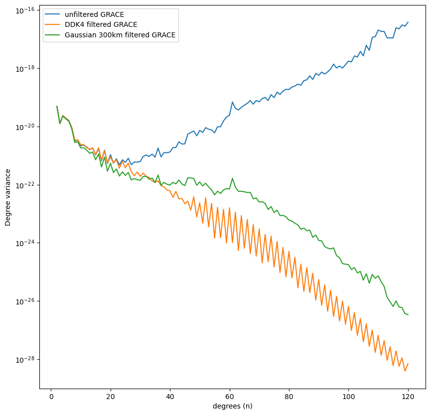
8. Spectral effect on a GRACE solution#
Besides the Anisotropic differences, the strength of the damping with degree shows a different behavior for the Gaussian versus Anisotropic filter. This can be seen from the plot below, where it is clear that the filters differ in the mid-degrees where the anisotropic filter retains more signal.
[10]:
gracetest="../../../tests/testdata/GSM-2_2008122-2008153_0030_EIGEN_G---_0004in.gz"
ds=xr.open_dataset(gracetest,engine='shascii').sh.truncate(120,2)
ds['cnmfilt']=ds.cnm.sh.filter('DDK4')
ds['gaussfilt']=ds.cnm.sh.filter('Gauss300')

dv=ds.cnm.sh.degvar()
filtdvt=ds.cnmfilt.sh.degvar()
gaussfiltdvt=ds.gaussfilt.sh.degvar()

fig, ax = mpl.subplots(figsize=(10, 10))

dv.plot(x='n',ax=ax,label="unfiltered GRACE")
filtdvt.plot(x='n',ax=ax,label="DDK4 filtered GRACE")
gaussfiltdvt.plot(x='n',ax=ax,label="Gaussian 300km filtered GRACE")
ax.legend()
ax.set_yscale('log')