Download this Jupyter notebook from github
Convert Geopandas GeoSeries to spherical harmonics#
Author: R. Rietbroek June 2025 (r.rietbroek@utwente.nl)*
Often, geographical geometry objects are needed as masks (1 inside,0 outside) expressed in the spherical harmonic domain. This notebook shows how a geopandas Geoseries, containing polygon masks or points can be converted to spherical harmonic coefficients
1. Preparations#
[1]:
#Optionally enable autoreloading for development purposes. Note that this does not automagically reload the binary extensions
%load_ext autoreload
%autoreload 2
[2]:
import xarray as xr
import os
import shxarray
import matplotlib.pyplot as plt
import cartopy.crs as ccrs

import numpy as np
import geopandas as gpd
from shapely import Point
[3]:
#set the maximum desired degree of the output spherical harmonics
nmax=120
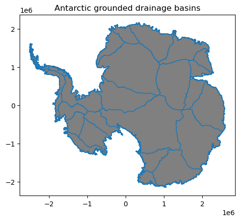
2. Get a set of Antartic grounded drainage basins (as polygons) to use as continental loads#
Note that in this case we load the geometries from a geoslurp database, but the example can be easily modified to load shapes from e.g. geopackage files.
[4]:
# In this example we're loading the drainage basin outlines froma geoslurp database
# The original datasources can be found at https://earth.gsfc.nasa.gov/cryo/data/polar-altimetry/antarctic-and-greenland-drainage-systems
from geoslurp.manager import GeoslurpManager
import geoslurp.tools.pandas
import pandas as pd
gsman=GeoslurpManager()

tname="cryo.antarc_ddiv_icesat_grnd"

# One can populate the database like this:
#dsant=gsman.dataset(tname)
#dsant.pull()
#dsant.register()

#load the polygons from the databse in a geopandas dataframe NOTE: convert to polar stereographic projection because the polgyon contains the south Pole
#And this projection is needed when converting to spherical harmonics
dfant=pd.DataFrame.gslrp.load(gsman.conn,f"SELECT basinid,ST_transform(geom::geometry,3031) as geometry FROM {tname}")
# quick plot of the drainage basin outlines
ax=dfant.plot(edgecolor="tab:blue",facecolor="grey")
ax.set_title("Antarctic grounded drainage basins")
[4]:
Text(0.5, 1.0, 'Antarctic grounded drainage basins')
3 Convert the drainage outline to spherical harmonics of the desired degrees#
We take the column basinid as an axiliary coordinate to indicate the original geometries present
[5]:
dantsh=xr.DataArray.sh.from_geoseries(dfant.geometry,nmax,auxcoord=dfant.basinid,engine="shtns")
dantsh.name='ant_div'
display(dantsh)

#optionally save to disk
fout=f"data/antarc_ddiv_icesat_grnd_n{nmax}.nc"
dantsh.reset_index('nm').to_netcdf(fout)
[SHTns 3.7.3] built Jan 17 2025, 23:35:53, id: v3.7-9-gbfb51b8*,avx2,ishioka,openmp,cuda
shxarray-INFO: Masking and gridding polygons
shxarray-INFO: Applying SH analysis
<xarray.DataArray 'ant_div' (basinid: 27, nm: 14641)> Size: 3MB
array([[ 9.40267020e-04, -3.05624425e-04, -1.59546257e-03, ...,
         0.00000000e+00,  0.00000000e+00,  0.00000000e+00],
       [ 1.54626069e-03, -4.34739860e-05, -2.67059892e-03, ...,
         0.00000000e+00,  0.00000000e+00,  0.00000000e+00],
       [ 3.05559875e-03,  1.44490204e-04, -5.21075910e-03, ...,
         0.00000000e+00,  0.00000000e+00,  0.00000000e+00],
       ...,
       [ 5.83668038e-05, -3.63363264e-05, -9.28618692e-05, ...,
         0.00000000e+00,  0.00000000e+00,  0.00000000e+00],
       [ 7.85327017e-05, -4.81902117e-05, -1.24477510e-04, ...,
         0.00000000e+00,  0.00000000e+00,  0.00000000e+00],
       [ 9.11249032e-05, -4.32464570e-05, -1.50067337e-04, ...,
         0.00000000e+00,  0.00000000e+00,  0.00000000e+00]])
Coordinates:
  * nm       (nm) object 117kB MultiIndex
  * n        (nm) int64 117kB 0 1 1 1 2 2 2 2 ... 120 120 120 120 120 120 120
  * m        (nm) int64 117kB 0 -1 0 1 -2 -1 0 1 ... 114 115 116 117 118 119 120
  * basinid  (basinid) float64 216B 2.0 3.0 4.0 5.0 6.0 ... 25.0 26.0 27.0 27.0
Attributes:
    Conventions:  CF-1.8
    source:       shxarray-1.3.3.dev5+ga1b06ac.d20250527 <https://github.com/...
    contact:      Roelof Rietbroek <r.rietbroek@utwente.nl>
    institution:  ITC Faculty of Geo-Information Science and Earth Observatio...
    comments:     Used backend: SHTns High performance Spherical Harmonic Tra...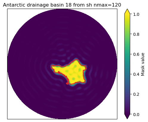
history: Analysis operation4 Check if the intermediate drainage basin results made sense#
A spatially discontinuous function cannnot be one-to-one mapped to spectrally truncated function, so some Gibb’s phenomena is to be expected
[6]:
# Sum all spherical harmonic coefficient sets for all basins and grid
import cartopy.crs as ccrs
dres=0.25
basinid=18
# basinid=3
daantgrd=dantsh.sel(basinid=basinid).sh.synthesis(lon=np.arange(-180+dres/2,180,dres),lat=np.arange(-90+dres/2,-60,dres))
daantgrd.name="Mask value"
# daantgrd=daantgrd[daantgrd.lat < -50]
ax = plt.axes(projection=ccrs.SouthPolarStereo())
daantgrd.plot(ax=ax,vmax=1,vmin=0,transform=ccrs.PlateCarree())
ax.add_geometries(dfant[dfant.basinid==basinid].geometry,edgecolor='tab:red',crs=ccrs.SouthPolarStereo(),facecolor="none",lw=2)
plt.title(f"Antarctic drainage basin {basinid} from sh nmax={nmax}")
[6]:
Text(0.5, 1.0, 'Antarctic drainage basin 18 from sh nmax=120')
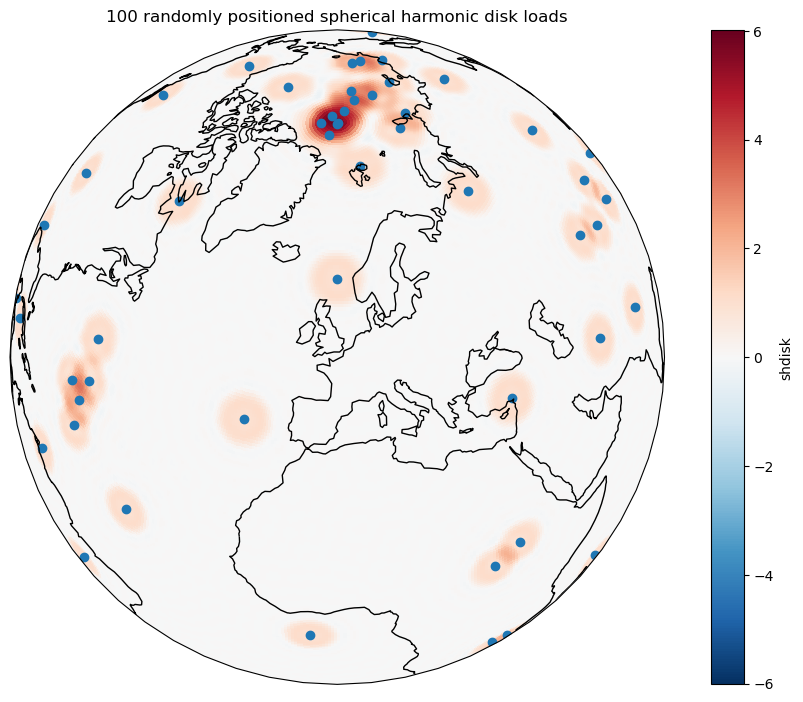
5 What about the conversion of geometry points?#
Points can be interpreted as unit loads, disks or parabolic loads, before being expanded into spherical harmonic coefficients. Let’s create some randomized points on the sphere first
[8]:
from random import sample
npoints=100
latrange=180
lonrange=360
discr=0.001245
latpnt=sample(sorted(np.arange(-90,90,discr)),npoints)
lonpnt=sample(sorted(np.arange(-180,180,discr)),npoints)
gspnts=gpd.GeoSeries([Point(x,y) for x,y in zip(lonpnt,latpnt)]).set_crs(ccrs.PlateCarree())
[9]:
#convert the points to spherical harmonics of disks with spherical radius of 4 degrees
dadskssh=xr.DataArray.sh.from_geoseries(gspnts,nmax,axialtype="disk",psi=4)

#unitload
#daunitsh=xr.DataArray.sh.from_geoseries(gspnts,nmax)

#Parabolic caps
# daparacsh=xr.DataArray.sh.from_geoseries(gspnts,nmax,axialtype="paraboliccap",psi=4)

display(dadskssh)
<xarray.DataArray 'shdisk' (nlonlat: 100, nm: 14641)> Size: 12MB
array([[ 2.29283487e-031, -3.72144720e-031,  4.66482478e-030, ...,
         9.77530206e-032, -1.22533167e-030, -1.88727029e-033],
       [-7.06215820e-007, -1.18353985e-007,  5.60879349e-007, ...,
         1.18895074e-006, -5.63443570e-006, -8.99602868e-007],
       [-2.07855784e-106,  1.53760622e-105,  2.36993858e-104, ...,
         2.67070659e-107,  4.11640543e-106, -6.30951488e-107],
       ...,
       [-6.12887002e-079,  3.12849010e-078,  4.72988986e-077, ...,
        -1.01129752e-079, -1.52895670e-078, -4.32212865e-079],
       [ 4.96342288e-084, -1.30835992e-083, -1.98875738e-082, ...,
        -2.00649489e-083, -3.04994937e-082,  1.54471775e-084],
       [ 8.02365744e-009, -3.17705376e-009,  2.00659788e-008, ...,
        -8.17421239e-009,  5.16275723e-008,  7.09402100e-010]])
Coordinates:
  * nm       (nm) object 117kB MultiIndex
  * n        (nm) int32 59kB 120 119 120 118 119 120 ... 118 119 120 119 120 120
  * m        (nm) int32 59kB -120 -119 -119 -118 -118 ... 118 118 119 119 120
    lon      (nlonlat) float64 800B 165.8 -136.2 164.1 ... 143.0 -140.4 -116.3
    lat      (nlonlat) float64 800B -53.63 -17.72 81.92 ... 76.21 77.53 -23.94
    id       (nlonlat) int64 800B 0 1 2 3 4 5 6 7 8 ... 92 93 94 95 96 97 98 99
Dimensions without coordinates: nlonlat6 Create a visualization of all the disk loads together#
[10]:
dadsks=dadskssh.sum("nlonlat").sh.synthesis()

proj=ccrs.NearsidePerspective(central_longitude=0.0, central_latitude=50, satellite_height=35785831)
fig, ax = plt.subplots(subplot_kw={'projection': proj},figsize=(12,8.5))

ax.coastlines()
dadsks.plot(ax=ax,transform=ccrs.PlateCarree())
gspnts.plot(ax=ax,transform=ccrs.PlateCarree())
ax.set_title("100 randomly positioned spherical harmonic disk loads")
plt.show()